Convergence [of backdrop] is usually faster if the average of each input variable over the training set is close to zero. Among others, one reason is that when the neural network tries to correct the error performed in a prediction, it updates the network by an amount proportional to the input vector, which is bad if input is large
.
- Assign centers of clusters in some point in space (random at first try, calculating the centroid of each cluster the rest of the time)
- Associate each point to the closest center.
A couple of ways to normalize data:
Feature scaling
 |
| Figure 1, normalization formula |
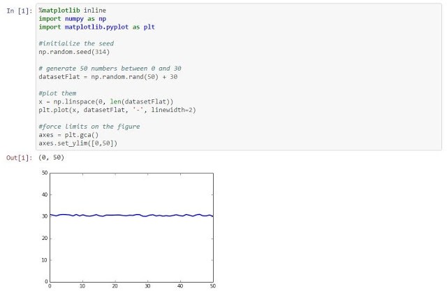 |
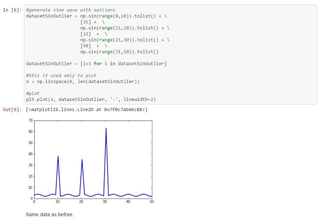
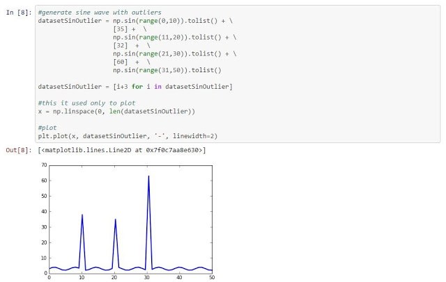
| Figure 2, Connection speed over 50 days |
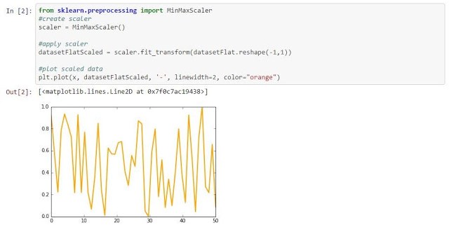 |
| Figure 3, Connection speed / day in scale 0-1. |
Standard scaler
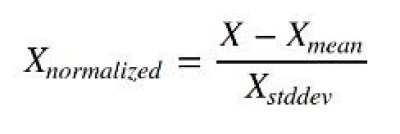 |
| Figure 4, Standard scaling formula |
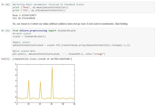 |
| Figure 6, Standard standardization for the above data is not a good choice. |
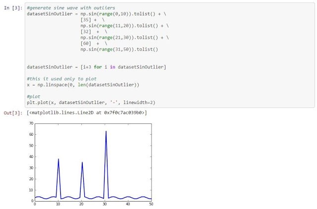
What happened? First, we were not able to scale the data between 0 and 1. Second, we now have negative numbers, which is not a dead end, but complicates the analysis. And third, now we are unable to clearly distinguish the differences between weekdays and weekends (all close to 0), because outliers have interfered with the data.
From a very promising data, we now have an almost irrelevant one. One solution to this situation could be to pre-process the data and eliminate the outliers (things change with outliers).
Scaling over the maximum value
The next idea that comes to mind is to scale the data by dividing it by its maximum value. Let´s see how it behaves with our data sets (sklearn.preprocessing.MaxAbsScaler).
 |
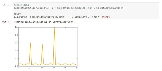
| Figure 7, data divided by maximum value |
 |
| Figure 8, data scaled over the maximum |
Good! Our data is in range 0,1… But, wait. What happened with the differences between weekdays and weekends? They are all close to zero! As in the case of standardization, outliers flatten the differences among the data when scaling over the maximum.
Normalizer
The next tool in the box of the data scientist is to normalize samples individually to unit norm (check this if you don’t remember what a norm is).
 |
| Figure 9, samples individually sampled to unit norm |
This data rings a bell in your head right? Let’s normalize it (here by hand, but also available as sklearn.preprocessing.Normalizer).
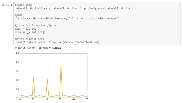 |
| Figure 10, the data was then normalized |
At this point in the post, you know the story, but this case is worse than the previous one. In this case we don’t even get the highest outlier as 1, it is scaled to 0.74, which flattens the rest of the data even more.
Robust scaler
The last option we are going to evaluate is Robust scaler. This method removes the median and scales the data according to the Interquartile Range (IQR). It is supposed to be robust to outliers.
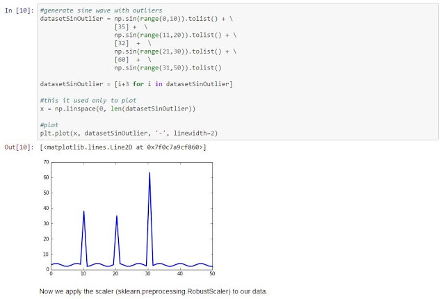 |
| Figure 11, the median data removed and scaled |
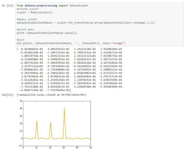 |
| Figure 12, use of Robust scaler |
You may not see it in the plot (but you can see it in the output), but this scaler introduced negative numbers and did not limit the data to the range [0, 1]. (OK, I quit).
There are others methods to normalize your data (based on PCA, taking into account possible physical boundaries, etc), but now you know how to evaluate whether your algorithm is going to influence your data negatively.
Things to remember (basically, know your data):
Normalization may (possibly [dangerously]) distort your data. There is no ideal method to normalize or scale all the data sets. Thus it is the job of the data scientist to know how the data is distributed, know the existence of outliers, check ranges, know the physical limits (if any) and so on. With this knowledge, one can select the best technique to normalize the feature, probably using a different method for each feature.
If you know nothing about your data, I would recommend you to first check the existence of outliers (remove them if necessary) and then scale over the maximum of each feature (while crossing your fingers).
Written by Santiago Morante, PhD, Data Scientist at LUCA Consulting Analytics
The post Warning About Normalizing Data appeared first on Think Big.
