We have finally come to the last part of the Machine Learning experiment with Python for all. We have been taking it step by step, and in this last post we will address any doubts and keep going through to the end. In this post we will select the algorithms, construct the models, and we will put our validation dataset to the test. We have built a good model, and above all, we have lost our fear of Python. And so…we´ll keep learning!
The steps that we have taken in the previous post are as follows:
- Load the data and modules/libraries we need for this example
- Explore the data
We will now go through the following:
- Evaluation of different algorithms to select the most adequate model for this case.
- The application of the model to make predictions from the ´learnt´
3. Selecting the algorithms
The moment has come to create models from the known data and estimate their precision with new data. For this, we´re going to take the following steps:
- We will separate part of the data to create a validation dataset
- We will use cross validation for 10 interactions to estimate accuracy
- We will build 5 different models to predict (from the measurements of the flowers collected in the dataset) which species the new flower belongs to
- We will select the best model
3.1 Creation of the validation dataset
How do we know if our model is good? To know what type of metrics we can use to evaluate the quality of a model based in Machine Learning, we recommend you read this post we published recently about the Confusion Matrix. We used statistical methods to estimate the precision of the models, but we also had to evaluate them regarding new data. For this, just as we did in the experiment before Machine Learning, this time in the Azure Machine Learning Studio, we will reserve 20% of the data from the original dataset. And so, applying this together with the validation, we can check how the model we have generated works, and the algorithm that we chose in this case with 80% remaining. This procedure is known as a holdout method.
With the following code, which, as we have done before, we can type or copy and paste into our Jupyter Notebook, separating the data into training sets X_train, Y_train and the validation ones X_validation, Y_validation.
This method is useful because its quick at the time of computing. However, its not very precise, as the results already vary a lot when we chose different training data. To overcome these issues, the concept of cross validation emerged.
3.2 Cross-validation
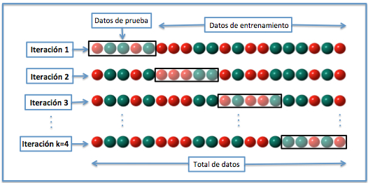
The objective of cross-validation is to guarantee that the results we obtain are independent from the partition between training data and validation data, and for this reason it is often used to validate models generate in AI projects. It consists of the repeating and calculating of the arrhythmic average of the evaluation methods that we obtain about different partitions. In this case, we are going to use a process of cross-validation with 10 interactions. This means that our collection of training data is divided into 10 parts, trained in 9, validated in 1, and the process repeated 10 times. In the image we can see a visual example the process with 4 interactions.

To evaluate the model, we chose the estimation variable scoring the accuracy metric that represents the ratio between the number of instances that the model has predicted correctly, against the number of total instances in the dataset, multiplied for 100 to give a percentage.
For this, we add the following code:
3.3 Constructing the models
As beforehand, we don’t know which algorithms work best for this problem, so we will try 6 different ones, lineal ones (LR, LDA), as well as non-lineal ones (KNN, CART, NB and SVM). The initial graphs indicated that we can imagine they will work, because some of the classes appear to be separated lineally in some dimension. We will evaluate the following algorithms:
- Logistic regression LR
- Lineal discrimination analysis LDA
- K-near neighbours KNN
- Classification and regression trees CART
- Naïve Bayes NB
- Support Vector Machines SVM
Before each execution we reset the initial (seed) value to make sure that the evaluation of each algorithm is made sure to be using to same collection of data (data split), to ensure that the results will be directly comparable. We will add the following code:
3.4 Choosing the model that works best
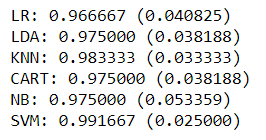
If we execute the cells (Cell/Run Cells) we can observe the estimations for each model. In this way we can compare them and chose the best. If we look at the results obtained, we can see that the model with the highest precision value is KNN (98%).

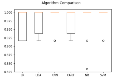
We can also create a graph of the results of the model evaluation and compare the distribution and average precision for each model (each algorithm is already evaluated in 10 interactions for the type of cross-validation that we have chosen). For this, we add the following code:
We get this result:

In the box and whisker diagram it is clear that the precision shown in many of the models KNN, NB and SVM are 100%, whilst the model that offers the least precision is the lineal regression LR.
4. Applying the model to make predictions
The moment has come to put the model we created to the test from the training data. For this, what we do its apply it to the original part of the dataset that we separate at the start as the validation dataset. As we have the correct classification values, and they have not been used in the training model, if we compare the real values with the predicted ones for the model we will see if the model is good or not. To do this we apply the chosen model (the one that gave us the best accuracy in the previous step) directly to this dataset, and we summarise the results with a final validation score, a confusion matrix and a classification report.
To apply the base model to the SVM algorithm, we don’t need to do any more than run the following code:
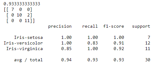
We get something like this:

As we can see, accuracy is 0.93 or 93%, a good result. The confusion matrix indicates that the number of points the prediction model got correct (diagonal values: 7+10+11=28), and the elements outside of the diagonal are the prediction errors (2). From this, we can conclude that it is a good model and we can apply it comfortably to our new dataset.
We have based the model on the SVM model, but the precision values for KNN are also very good. Are you excited to do this last step and apply the other algorithm?
With this step ,we can officially say that we have finished our first Machine Learning experiment with Python. Our recommendation: re-do the whole experiment, taking notes of any doubts that arise, try to look for the answers, try to make small changes to the code, like the last one we proposed and… Across platforms such as Coursera, edX, DataCamp or CodeAcademy, you can find free courses to keep getting better. Never stop learning!
Other posts from this tutorial:
- Dare with Python: An experiment for all (intro)
- Python for all (1): Installation of the Anaconda environment.
- Python for all (2): What are the Jupiter Notebook ?. We created our first notebook and practiced some easy commands.
- Python for all (3): ScyPy, NumPy, Pandas…. What libraries do we need?
- Python for all (4): We start the experiment properly. Data loading, exploratory analysis (dimensions of the dataset, statistics, visualization, etc.)
- Python for all (5) Final: Creation of the models and estimation of their accuracy
Don’t miss out on a single post. Subscribe to LUCA Data Speaks.
You can also follow us on Twitter, YouTube and LinkedIn
The post Python for all (5): Finishing your first Machine Learning experiment with Python appeared first on Think Big.